How out-of-the-box sampling can fail and how to fix it
Most data scientists rely on out-of-the-box sampling methods such as optimizing with stochastic gradient descent or cross-validating their models. However, these naive sampling methods can sometimes lead data scientists astray with biased results. Luckily, with a little statistical theory and geometry, we can determine when to naively sample, and when we need to be a bit more clever.
Experiment
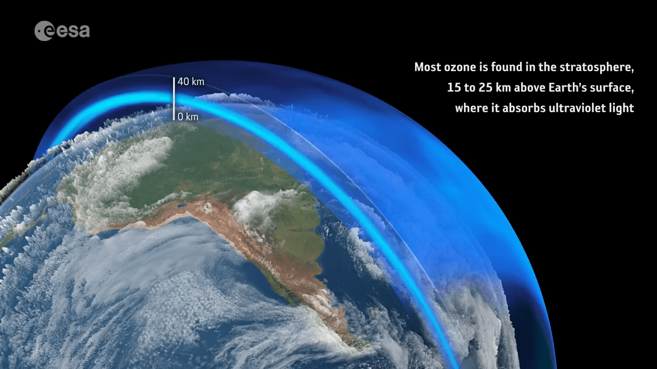
Suppose you’re an amateur climatologist who wants to determine if there is any new damage to the ozone layer. You can’t check every atmospheric point (satellite usage is expensive!) so you sample 1000 points on the Earth’s stratosphere. How should you pick those points?
To pick each point, we can use 3D spherical coordinates to ensure that each of the sampled points are on the surface of the sphere.
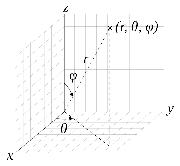
\[x = r sin(\phi)cos(\theta)\] \[y = r sin(\phi)sin(\theta)\] \[z = rcos(\phi)\] \(x, y, z\) are all on the surface of the sphere for a constant \(r\). I will normalize \(r\) to 1 for the rest of this post.
Naive sampling
Intuitively, one would think sampling uniformly on \(\theta\) and \(\phi\) would result in the points being uniformly distributed on the sphere. Unfortunately, the points tend to cluster at the north and south poles \((z = \pm 1)\), creating a biased sample. You can interact with the plot below to better see the clustering at the poles.
library(dplyr)
library(latex2exp)
library(plotly)

n <- 1000

theta_est_naive <- runif(n, min = 0, max = 2 * pi)
phi_est_naive <- runif(n, min = 0, max = pi)

x_est_naive <- sin(phi_est_naive) * cos(theta_est_naive)
y_est_naive <- sin(phi_est_naive) * sin(theta_est_naive)
z_est_naive <- cos(phi_est_naive)

p_naive <- plot_ly(
  x = x_est_naive,
  y = y_est_naive,
  z = z_est_naive,
  alpha = 0.75,
  type = "scatter3d",
  mode = "markers",
  size = 0.001,
) %>%
  layout(
    title = "Naive sampling on Sphere",
    scene = list(camera = list(eye = list(x = 0.6, y = 0.8, z = 1.25))),
    annotations = list(
      x = 1, y = -0.1,
      text = paste(
        "Click and drag to move the camera,",
        "zoom with scroll-wheel"
      ),
      showarrow = F, xref = "paper", yref = "paper",
      xanchor = "right", yanchor = "auto", xshift = 0, yshift = 0,
      font = list(size = 15, color = "red")
    )
  )
widgetframe::frameWidget(p_naive)
To explain why we get these results, let’s look at a 2d circle. While the data is distributed uniformly between the angles \(\theta\) and \(\phi\), the space between each point is being stretched as the points move away from the center of the circle. The stretching generalizes to higher dimensions as shown previously with the clustering at the poles.
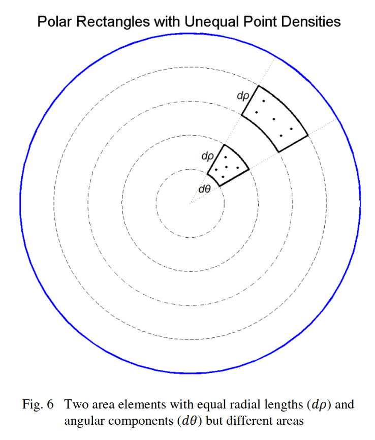
Mathematically, the proof of clustering at the poles on a sphere is shown by: \[ A = \int^{2\pi}_0 \int^{\pi}_0 sin\phi d\phi d\theta\] \[\implies dA = sin(\phi) d\phi d\theta\] The marginal area is a function of \(\phi\) which implies that the area density of uniformly random points is not constant. Notice that the \(\phi\) in the marginal area equation is minimized at \(\phi = \{0, \pi\}\). In Cartesian coordinates, that corresponds to the North and South poles, respectively (\(z \pm 1\)). The marginal area will hence correspondingly get smaller at the two poles. Therefore, if points are uniformly sampled in each marginal area, the poles are more area-dense as compared to points sampled from the equator. To achieve uniform samples throughout the sphere, we need our sampling method to incorporate how the marginal area changes along the surface area.
Sampling with theory
So how do we de-bias the sample? While there are many different ways to correctly sample, I will use \(\underline{\textbf{inverse transform sampling}}\) only because in this example we can derive the CDF and each sample is expensive to obtain. In other conditions, rejection sampling methods such as MCMC may be more appropriate.
We first need to find a suitable pdf. Suppose \(v\) is a point on the sphere \(S\). We need to construct a pdf such that the probability density is constant throughout the sphere. We can use a couple facts about probability and the sphere’s geometry to find \(f(v)\).
- Points can only be sampled on the surface of the sphere. \[\int\int_S f(v) dA = 1\]
- The surface area of the sphere is: \[\int\int_S dA = \int_0^{2\pi} \int_0^{\pi} sin(d\phi) d\phi d\theta = 4 \pi\]
Hence, \[f(v)dA = f(\theta, \phi) d\theta d\phi \implies f(\theta, \phi) = \frac{1}{4\pi}sin(\phi)\] We can find the marginal distribution of \(\theta\), and \(\phi\) from the joint distribution by: \[f(\theta) = \int_0^\pi \frac{1}{4\pi}sin(\phi) d\phi = \frac{1}{2\pi}\]
\[f(\phi) = \int_0^{2\pi} \frac{1}{4\pi}sin(\phi) d\theta = \frac{sin(\phi)}{2}\]
Notice that the first equation is already a constant so we don’t need to transform it. The second equation is a function of \(\phi\) and requires a transformation. Remember that \(\phi\) refers to the polar angle where \(\phi = 0, \pi\) point to the poles \(z \pm 1\). Hence, we only need to adjust how we sample \(\phi\) to correct the bias.
We can now use inverse transform sampling. The first step is to find the CDF of \(f(\phi)\): \[F(\phi_0) = \int_0^{\phi_0} \frac{sin(\phi)}{2} d\phi = \frac{1}{2}(1 - cos(\phi_0)) \] Then, we find the inverse of the CDF: \[F^{-1}(u) = arccos(1 - 2u) \] Lastly, we uniformly sample \(u\) and transform it based on the inverse CDF above: \[U \sim unif(0,1)\] \[X \sim arccos(1 - 2U)\] The transformed distribution \(X\) will conform to the wanted pdf \(f(\phi)\).
theta_est <- runif(n, min = 0, max = 2 * pi)
phi_est <- sapply(runif(n), function(u) acos(1 - 2 * u))

x_est <- sin(phi_est) * cos(theta_est)
y_est <- sin(phi_est) * sin(theta_est)
z_est <- cos(phi_est)

p2 <- plot_ly(
  x = x_est,
  y = y_est,
  z = z_est,
  alpha = 0.75,
  type = "scatter3d",
  mode = "markers",
  size = 0.001
) %>%
  layout(
    title = "Uniform sampling on Sphere",
    scene = list(camera = list(eye = list(x = 1.25, y = 0.25, z = 0.75))),
    annotations = list(
      x = 1, y = -0.1,
      text = paste(
        "Click and drag to move the camera,",
        "zoom with scroll-wheel"
      ),
      showarrow = F, xref = "paper", yref = "paper",
      xanchor = "right", yanchor = "auto", xshift = 0, yshift = 0,
      font = list(size = 15, color = "red")
    )
  )
widgetframe::frameWidget(p2)
tl;Dr
Probability problems routinely go against intuition, even more so at high dimensions. Sometimes machine learning is not enough and you’ll need probability theory to carry the day.
For an encyclopedic amount of different methods to generate uniformly random points on n-spheres and in n-balls go to extreme learning.
Citations:
Arthur, Mary K. 2015. “Point Picking and Distributing on the Disc and Sphere.” Army Research Laboratory. https://apps.dtic.mil/dtic/tr/fulltext/u2/a626479.pdf.