Exploring the data

library(readr)
library(ggplot2)
library(stringr)
library(tidyr)
library(dplyr)
library(forcats)
library(fuzzyjoin)
library(stringdist)
library(tigris)
library(plotly)

beer_styles <- read_csv("beer_styles.csv")

state_info <- fips_codes %>%
  group_by(state) %>%
  slice(1) %>%
  select(state, state_name)

beer_awards <- readr::read_csv(
  paste0("https://raw.githubusercontent.com/rfordatascience/tidytuesday/",
         "master/data/2020/2020-10-20/beer_awards.csv")) %>%
  mutate(brewery = str_replace(brewery, " Company", ""),
         brewery = str_replace(brewery, " Co.", ""))

beers <- read_csv("beers.csv") %>%
  select(-X1)
breweries <- read_csv("breweries.csv") %>% 
  mutate(name = str_replace(name, " Company", ""),
         name = str_replace(name, " Co.", "")) %>%
  inner_join(state_info, by="state")

beer_joined <- breweries %>%
  inner_join(beers, by="brewery_id") %>%
  rename(brewery_name = name.x,
         beer_name = name.y) %>%
  full_join(beer_awards,
            by=c("city"="city",
                 "state"="state",
                 "brewery_name"="brewery",
                 "beer_name"="beer_name")) %>%
  inner_join(state_info, by="state") %>%
  mutate(state_name = if_else(is.na(state_name.x),
                              state_name.y, state_name.x)) %>%
  select(-state_name.x, -state_name.y) %>%
  rename(style2 = style)

beer_awards_joined <- beer_joined %>%
  mutate(category = case_when(
    is.na(category) & !is.na(style2) ~ style2,
    is.na(category) & is.na(style2) ~ beer_name,
    TRUE ~ category)) %>%
  mutate(category = str_replace_all(category, "-", " "),
         category = str_replace_all(category, "Ale, ", ""),
         category = str_replace_all(category, "Lager, ", "")) %>%
  select(-id, -style2) %>%
  stringdist_left_join(beer_styles, by = c("category"="category")) %>%
  mutate(category = str_to_lower(if_else(is.na(category.x), category.y, category.x))) %>%
  select(-category.y, -category.x) %>%
  mutate(category = case_when(
    str_detect(category, "dry stout") &
      !str_detect(category, "irish") ~ "dry stout",
    str_detect(category, "foreign style|export") &
      style == "Stouts" ~ "foreign style stout",
    TRUE ~ category),
    style = case_when(
      str_detect(category, "brown") ~ "Brown Ales",
      str_detect(category, "dark lager|o*tober|dark pils") ~ "Dark Lagers",
      str_detect(category, "dark ale") ~ "Dark Ales",
      str_detect(category, "gose|wild|fruit|brett|sour") ~ "Wild/Sour Beers",
      str_detect(category, "wheat|style weisse") ~ "Wheat Beers",
      str_detect(category, "cream") ~ "Hybrid Beers",
      str_detect(category, "spice|special|alcoholic") ~ "Specialty Beers",
      str_detect(category, "pils|bitter|amber ale|light lager|zwickelbier|helles") ~ "Pale Ales",
      str_detect(category, "pale ale") & !str_detect(category, "india") ~ "Pale Ales",
      str_detect(category, "strong ale") ~ "Strong Ales",
      str_detect(category, "india pale ale") ~ "India Pale Ales",
      TRUE ~ style)) %>%
  filter(!((category == "American IPA") & (style == "American IPA"))) %>%
  mutate(winner = !is.na(medal),
         category = str_to_title(category)) %>%
  filter(winner) %>%
  distinct()

With so many beer categories (448) there are only on average 11.1 beers in each category. With such a low sample size per beer category, the statistical power will be too low to apply time series or geospatial models, given they additionally reduce the sample size per bucket. As such, we can aggregate beer category to beer style, as defined by Beer Advocate, to created larger buckets and increase the sample size per bucket. The corresponding larger set of beers has only 15 different buckets with on average 343.43 beers in each beer style. As we then cut on state (50+1) and time (1987 - 2020), we can be assured that enough data will be within most buckets so that the analysis has sufficient power.

library(dplyr)
library(forcats)
library(ggplot2)
library(cowplot)

counts <- beer_awards_joined %>%
  mutate(style = if_else(is.na(style), " NA", style)) %>%
  group_by(style) %>%
  summarise(total_counts=n())

counts_total <- beer_awards_joined %>%
  mutate(style = if_else(is.na(style), " NA", style)) %>%
  count(style, category) %>%
  group_by(style) %>%
  summarise(num_of_beer_cat = n()) %>%
  inner_join(counts, by="style")

counts_total %>%
  ggplot() +
  aes(y=fct_reorder(style, desc(style)), x=total_counts,
      fill=fct_reorder(style, desc(style))) +
  geom_col(position = "dodge") +
  geom_text(aes(label=paste0("Buckets: ", num_of_beer_cat)),
            size=3.5, nudge_x = -45, nudge_y = -0.25) +
  theme_ipsum_ps(axis_title_size = 15, plot_title_size = 25) +
  labs(x = "# of Medals Awarded", y = "Beer Styles",
       title = "Medals Awarded per Beer Styles", 
       caption = "Buckets: Number of different Beer Categories") +
  theme(legend.position = "none") +
  scale_fill_manual(values = getPalette(15))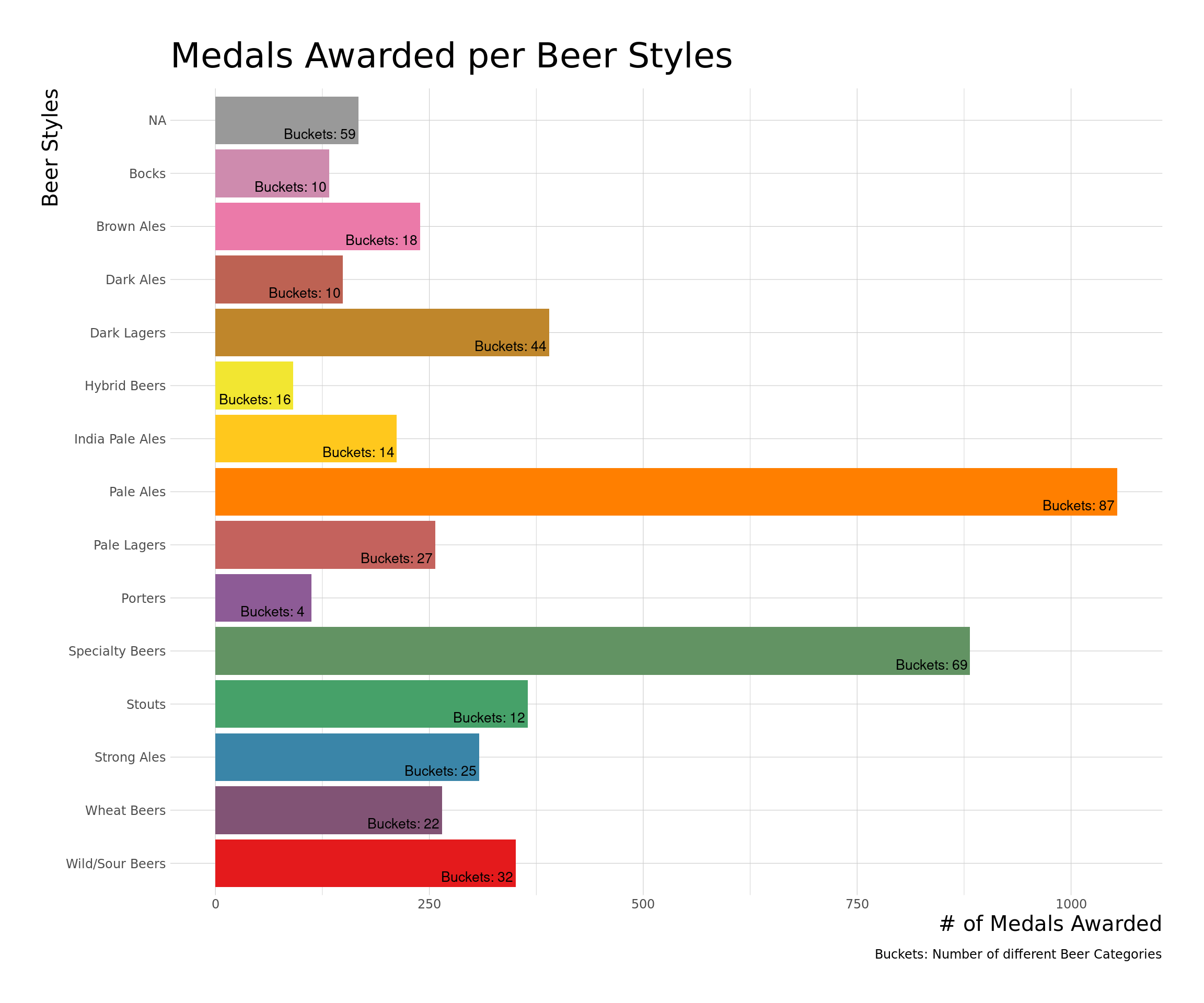

library(plotly)
viz <- beer_awards_joined %>%
  add_count(year, name = "year_total") %>%
  count(style, year, year_total, sort = TRUE) %>%
  mutate(pct_year = n / year_total) %>%
  ggplot() +
  aes(y=pct_year, x=year, color=style, group=style,
      text = paste0(style, ": ", year, "\nCount: ", n)) +
  geom_point() +
  geom_line() +
  scale_y_continuous(labels = scales::percent_format(accuracy=1)) +
  theme_ipsum_ps(axis_title_size = 15, plot_title_size = 25) +
  labs(x = "Year", y = "", color = "Beer Style", 
       title = "% of Medals Awarded to Beer Style over Time") +
  scale_color_manual(values = getPalette(15))
ggplotly(viz, tooltip = "text")

Only Pale Ale, Specialty Beers, and recently, Wild/Sour Beers are the only beer styles which are differentiable in terms of medals awarded from the rest.

viz_state <- beer_awards_joined %>%
  filter(fct_lump(state, 10) != "Other") %>%
  add_count(year, name = "year_total") %>%
  count(state, year, year_total, sort = TRUE) %>%
  mutate(pct_year = n / year_total) %>%
  ggplot() +
  aes(y=pct_year, x=year, color=state, group=state,
      text = paste0(state, ": ", year, "\nCount: ", n)) +
  geom_point() +
  geom_line() +
  scale_y_continuous(labels = scales::percent_format(accuracy=1)) +
  theme_ipsum_ps(axis_title_size = 15, plot_title_size = 25) +
  labs(x = "Year", y = "", color = "State", 
       title = "% of Medals Awarded to Breweries in a\nState over Time") +
  scale_color_manual(values = getPalette(15))
ggplotly(viz_state, tooltip = "text")

Modeling

One would imagine that different states may specialize in different categories or styles of beer. We can model this using Log Odds which creates a statistic of the strength of the relationship between two events. In our example, we might ask what beer categories are over/under represented in a given state. This may indicate a beverage specialization and perhaps a consumer preference for that state.

library(tidylo)
library(tidytext)
library(tidyr)

log_odds <- beer_awards_joined %>%
  filter(fct_lump(category, 8) != "Other",
         fct_lump(state, 4) != "Other") %>%
  count(state, category, style) %>%
  complete(state, category, fill = list(n=0)) %>%
  bind_log_odds(state, category, n, uninformative = TRUE, unweighted = TRUE) %>%
  mutate(category = reorder_within(category, log_odds_weighted, state),
         style = if_else(is.na(style), "Bocks", style))


log_odds %>%
  ggplot() +
  aes(x=log_odds_weighted, y=category, fill=style) +
  geom_col() +
  scale_y_reordered() +
  facet_wrap(~ state, nrow = 4, scale = "free_y") +
  labs(y = "Beer Category", x = "Weighted Log Odds", fill = "Beer style",
       title = "Over/Under representation of different beer categories\n per US State",
       caption = "Positive Log Odds = Over represented\nNegative Log Odds = Under represented\n") +
  theme_ipsum_ps(axis_title_size = 15, plot_title_size = 20) +
  scale_fill_manual(values = getPalette(8))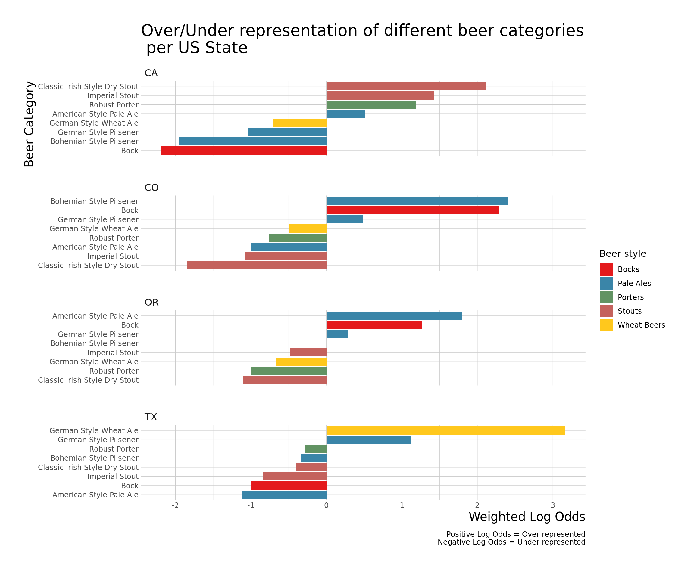

The analysis suggest that beer categories: Irish Dry and Imperial are more likely to come from California while Bock and (German/Bohemian) Pilseners are more likely to come from Colorado. Interestingly, some of the states have strong reversals in their log odds in comparison to other states suggesting states are specializing in their beers.

We can also specifically look at beer styles to check the robustness of the claim.

beer_awards_joined %>%
  filter(fct_lump(state, 4) != "Other",
         fct_lump(style, 8) != "Other") %>%
  count(state, style) %>%
  complete(state, style, fill = list(n=0)) %>%
  bind_log_odds(state, style, n) %>%
  mutate(style = reorder_within(style, log_odds_weighted, state),
         beer_style = sub("__.*", "", style)) %>%
  ggplot() +
  aes(x=log_odds_weighted, y=style, fill=beer_style) +
  geom_col() +
  scale_y_reordered() +
  facet_wrap(~ state, nrow = 4, scale = "free_y") +
  labs(y = "Beer style", x = "Weighted Log Odds", fill = "Beer style",
       title = "Over/Under representation of different beer styles\n per US State.",
       caption = "Positive Log Odds = Over represented\nNegative Log Odds = Under represented\n") +
  theme(text = element_text(size = 15)) +
  theme_ipsum_ps(axis_title_size = 15, plot_title_size = 25) +
  scale_fill_manual(values = getPalette(8))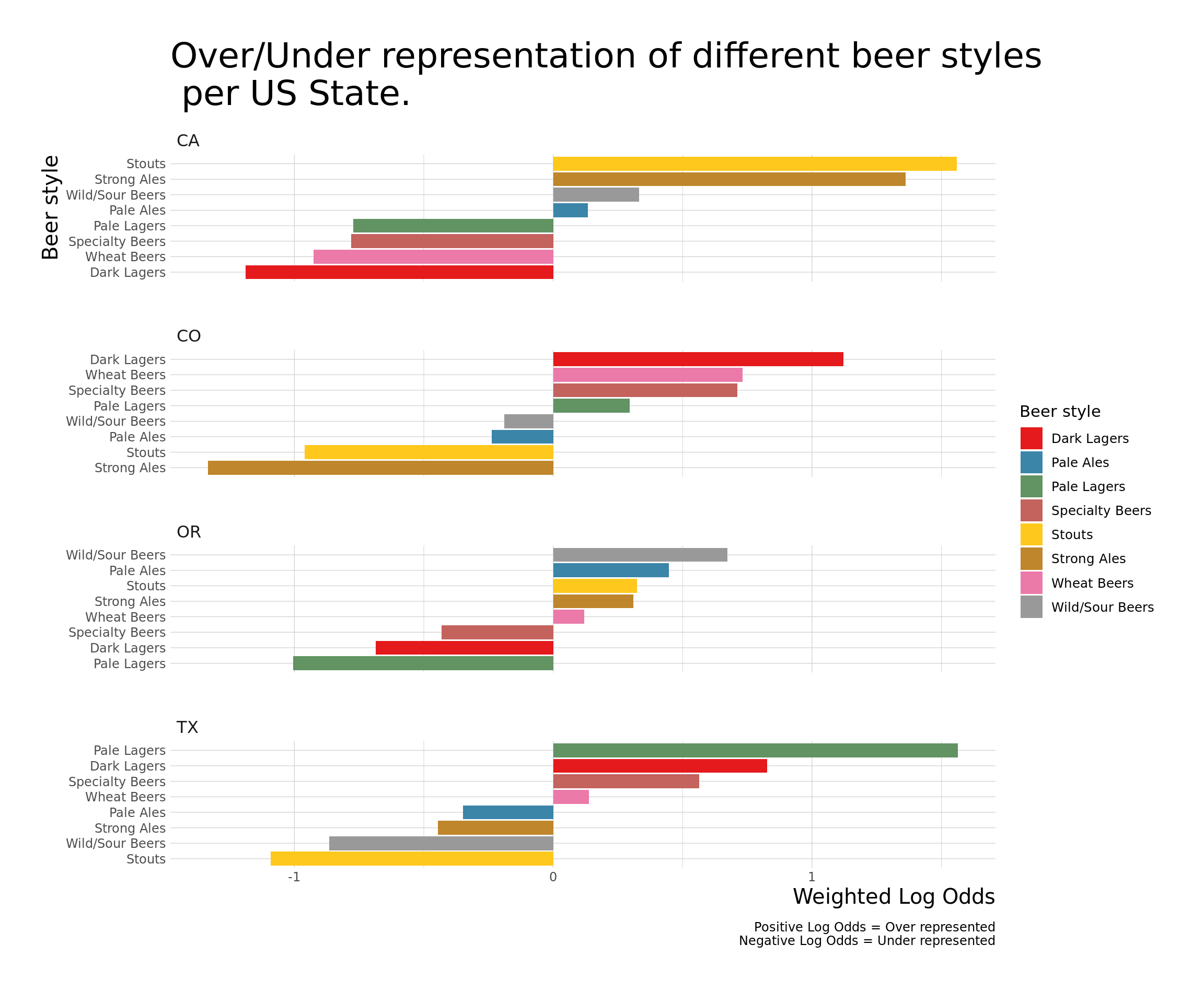

Aggregating the data still shows evidence of beer specialization per state. Some aspects of the specialization claim were over-stated as the Robust Porter is over-represented in California, however, Porters in general are not. Various specific categories of Wheat Beers are only vaguely over/under represented, however, the beer style of Wheat Beers are over-represented in Colorado and under-represented in California. Alternatively, in Texas, the German Style Wheat Ale is very over represented however, Wheat Beers in general are not. The Dark Lagers beer style is very over-represented in Colorado and Texas and are very under-represented in California and Oregon. However, no specific category of Dark Lagers is particularly over/under represented.

We can also view this plot throughout the US as a proxy for larger specialization zones (e.g West Coast, East Coast, etc.) in the US.

library(geofacet)
beer_awards_joined %>%
  filter(style %in% c("Dark Lagers", "Pale Ales", "Specialty Beers", "Stouts",
                      "India Pale Ales", "Strong Ales", "Wheat Beers", "Wild/Sour Beers")) %>%
  count(state, style) %>%
  complete(state, style, fill = list(n=0)) %>%
  bind_log_odds(state, style, n) %>%
  mutate(style = reorder_within(style, log_odds_weighted, state),
         beer_style = sub("__.*", "", style)) %>%
  ggplot() +
  aes(x=log_odds_weighted, y=reorder(beer_style, desc(beer_style)), fill=beer_style) +
  geom_col() +
  facet_geo(~ state, grid = "us_state_grid2") +
  scale_y_reordered() +
  theme_bw() +
  scale_fill_manual(values = getPalette(12)) +
  labs(x="Weighted Log-Odds", y="Beer Styles", fill="Beer Styles",
       title = "Weighted Log-Odds of different Beer Styles throughout the US",
       caption = "Positive Log Odds = Over represented\nNegative Log Odds = Under represented\n")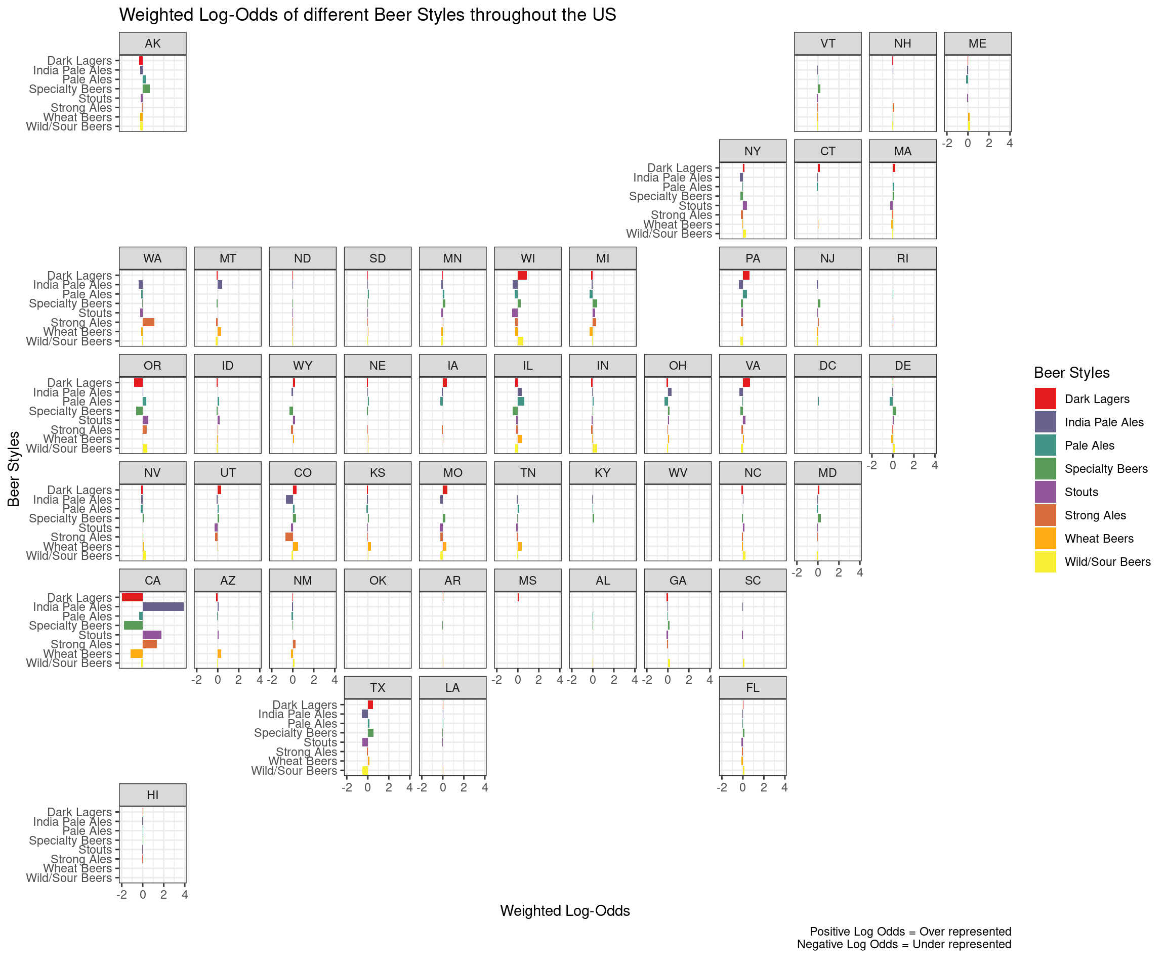

In short, we see not only evidence of state specialization but also regional specialization. The West Coast with California, Oregon, and Washington all have over representation in Strong Ales, and Stouts, while under representing Pale Lagers, and Dark Lagers. Only New York also over-represents Stout style beers. The Midwest to Appalachian regions are more varied in beer styles represented, however, Dark Lagers and Pale Lagers have strong presences. Texas has a similar profile of awarded beer styles to the Midwest than the West Coast.

Lastly, we can regress number of specific beer styles by year and state by year to compare whether the newer awards are being driven by beer style preferences or state preferences.

library(broom)
library(dplyr)
library(purrr)
by_year_style <- beer_awards_joined %>%
  add_count(year, name = "year_total") %>%
  count(style, year, year_total, sort = TRUE) %>%
  mutate(pct_year = n / year_total)

over_under <- by_year_style %>%
  group_by(style) %>%
  summarize(model = list(glm(cbind(n, year_total - n) ~ year, family = "binomial"))) %>%
  mutate(tidied = map(model, tidy, conf.int = TRUE)) %>%
  unnest(tidied) %>%
  filter(term == "year") %>%
  mutate(p.value = format.pval(round(p.value, 2)),
         style = fct_reorder(style, estimate))

over_under %>%
  ggplot() +
  aes(x=estimate, y=style) +
  geom_point(size=3) +
  geom_vline(xintercept = 0, lty = 2, color="red") +
  geom_errorbarh(aes(xmin = conf.low, xmax = conf.high), height = .1, size=1) +
  theme_bw() +
  labs(x = "Estimated slope",
       title = "Which beers styles are increasingly winning more\nAwards over time throughout the US?",
       y = "") +
  theme(text = element_text(size = 15)) +
  theme_ipsum_ps(axis_title_size = 15, plot_title_size = 25)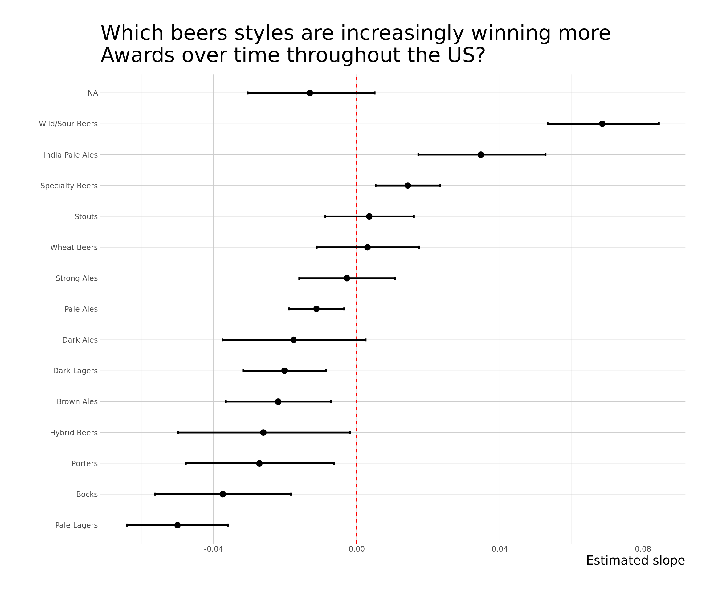

library(broom)
library(dplyr)
library(purrr)
by_year_state <- beer_awards_joined %>%
  add_count(year, name = "year_total") %>%
  count(state, year, year_total, sort = TRUE) %>%
  mutate(pct_year = n / year_total) 

over_under_state <- by_year_state %>%
  group_by(state) %>%
  summarize(model = list(glm(cbind(n, year_total - n) ~ year, family = "binomial"))) %>%
  mutate(tidied = map(model, tidy, conf.int = TRUE)) %>%
  unnest(tidied) %>%
  filter(term == "year") %>%
  mutate(p.value = format.pval(round(p.value, 2)),
         state = fct_reorder(state, estimate))

over_under_state %>%
  filter(state!="MS" &
           (estimate > quantile(estimate, 0.85) |
              estimate < quantile(estimate, 0.15))) %>%
  ggplot() +
  aes(x=estimate, y=state) +
  geom_point(size=3) +
  geom_vline(xintercept = 0, lty = 2, color="red") +
  geom_errorbarh(aes(xmin = conf.low, xmax = conf.high), height = .1, size=1) +
  theme_bw() +
  labs(x = "Estimated slope",
       title = "Which States are increasingly winning more Awards\n over time throughout the US?",
       y = "") +
  theme(text = element_text(size = 15)) +
  theme_ipsum_ps(axis_title_size = 15, plot_title_size = 25)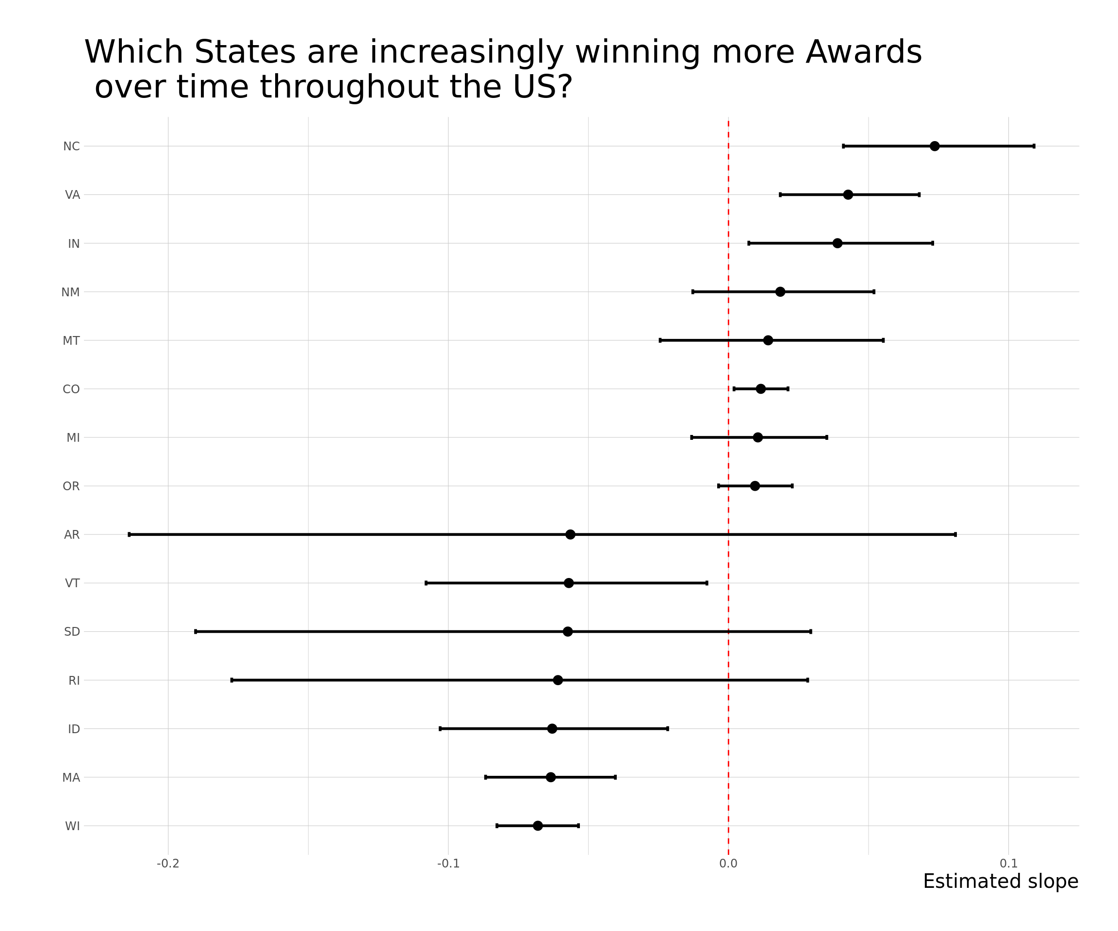

Conclusion

Wild/Sour Beers style are a clear up-and-coming beer award-winner. An interesting note is that if we return to the previous figure, Wild/Sour Beers style have marginal state level over representation throughout the US. Similarly, Specialty Beer is generally not under nor over represented anywhere except where it’s under-represented in California and in Oregon. On the other hand, India Pale Ales seems mostly driven by breweries in California. This indicates that changes in beer style preferences rather than changes in state preferences is driving the changes.

The is some evidence of specialization on the West Coast with Stouts and Strong Ales being over-represented, however, most specialization is solely at the state level - nearby states are equally variable to far away states. Moreover, there is some evidence of regional specialization in under-represented beer styles. In other words, Dark Lagers and Specialty Beers are under-represented in the West Coast while India Pale Ales are under-represented in Texas, Colorado, and Wisconsin.